The Central Limit Theorem
Understanding the Central Limit Theorem (CLT) — and How It Relates to the Law of Large Numbers
The Central Limit Theorem (CLT) is one of the most powerful and beautiful ideas in all of statistics. If the Law of Large Numbers explains why averages stabilize, the CLT explains what the distribution of those averages looks like—and why so many real‑world numbers end up following a bell curve.
Let’s break it down in a friendly, intuitive way.
What Is the Central Limit Theorem?
The Central Limit Theorem says:
If you take many random samples from any population and compute the average of each sample,
the distribution of those averages will form a normal (bell‑shaped) curve—
even if the original data is not bell-shaped.
In simpler words:
- Your raw data might be messy, skewed, or weirdly shaped
- But the averages of repeated samples tend to look beautifully normal
And this happens as long as your sample size is reasonably large (often n ≥ 30 is enough).
A Cookie‑Friendly Example
Imagine you have a huge batch of cookies that vary in weight.
- Individual cookies might follow any distribution—maybe most are heavy, some are light
- Now take groups of 30 cookies at a time, and calculate the average weight of each group
- If you repeat this over and over, the histogram of those averages will approach a normal curve
This is the CLT at work.
Why the CLT Is So Important
The CLT is the reason we can:
- Use normal‑based confidence intervals
- Run many hypothesis tests
- Build margins of error in polling
- Predict behavior in large systems
- Trust analytics in business intelligence
It’s the “why this works” behind a huge portion of statistical inference.
How the CLT Relates to the Law of Large Numbers (LLN)
The Law of Large Numbers and Central Limit Theorem are closely connected, but they answer different questions.
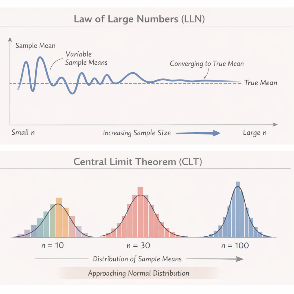
1. What the LLN tells us
As sample size increases, the sample mean converges to the true population mean.
It guarantees accuracy.
2. What the CLT tells us
As sample size increases, the distribution of sample means becomes normal.
It explains shape and variability.
Think of it this way:
| Concept | What It Explains | Example |
|---|---|---|
| LLN | The average will settle close to the true mean | The more you flip a coin, the closer to 50% heads you get |
| CLT | The distribution of many sample averages looks normal | If you collect many sets of 30 coin flips and record the % heads each time, those percentages form a bell curve |
Their relationship
- LLN: “Your average is likely close to the truth.”
- CLT: “And here’s the shape and spread of those averages.”
Together they explain why big samples are both accurate and predictable.
Real‑World Analogy: Driving on the Highway
The Law of Large Numbers is like cruise control:
- Over long distances, your average speed stabilizes, even if speed fluctuates moment to moment.
The Central Limit Theorem is like your GPS’s ETA predictions:
- They use a model that assumes the distribution of travel times behaves in a predictable, bell‑curved way across many trips.
Different ideas, working together to explain stability and predictability.
Summary
Law of Large Numbers
- Focus: long‑run average
- Claim: Averages get closer to the true value with more data
Central Limit Theorem
- Focus: distribution of averages
- Claim: Averages from many samples follow a bell curve
How they connect
- LLN ensures averages approach truth
- CLT explains the variability and shape of those averages
- Together, they make statistical inference possible